How To Add Lines To A Scatter Plot On Excel

Note:The following procedure applies to Office 2013 and newer versions. Office 2010 steps?

Create a scatter chart

And then, how did nosotros create this besprinkle nautical chart? The following procedure will help you create a scatter chart with similar results. For this nautical chart, we used the example worksheet data. You tin can re-create this data to your worksheet, or y'all tin use your own data.

1. Copy the example worksheet data into a blank worksheet, or open the worksheet that contains the data you lot desire to plot in a scatter chart.

   1 ii iii four 5 half dozen 7 viii 9 10 11

   A B Daily Rainfall Particulate 4.1 122 4.3 117 v.7 112 5.4 114 v.nine 110 5.0 114 3.six 128 ane.9 137 vii.iii 104

2. Select the data you lot want to plot in the scatter chart.

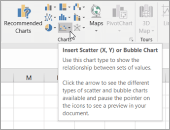
3. Click the Insert tab, and so click Insert Scatter (X, Y) or Chimera Nautical chart.

   

4. Click Besprinkle.

   Tip:You tin can rest the mouse on whatsoever nautical chart type to see its name.

5. Click the chart area of the chart to display the Design and Format tabs.

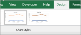
6. Click the Design tab, so click the chart way you want to apply.

   

7. Click the chart title and type the text you desire.

8. To modify the font size of the nautical chart championship, right-click the title, click Font, and and so enter the size that you lot want in the Size box. Click OK.

9. Click the nautical chart area of the nautical chart.

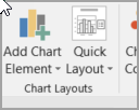
10. On the Pattern tab, click Add together Chart Element > Centrality Titles, and and then do the following:

    

    1. To add together a horizontal axis title, click Chief Horizontal.

    2. To add a vertical centrality title, click Primary Vertical.

    3. Click each championship, blazon the text that you want, and then printing Enter.

    4. For more title formatting options, on the Format tab, in the Chart Elements box, select the title from the list, and so click Format Option. A Format Title pane will announced. Click Size & Properties , and then you can choose Vertical alignment, Text direction, or Custom angle.

11. Click the plot expanse of the chart, or on the Format tab, in the Chart Elements box, select Plot Expanse from the list of chart elements.

    

12. On the Format tab, in the Shape Styles group, click the More button , and so click the effect that you want to employ.

13. Click the nautical chart expanse of the chart, or on the Format tab, in the Chart Elements box, select Nautical chart Area from the list of nautical chart elements.

14. On the Format tab, in the Shape Styles group, click the More than push , and and then click the effect that you want to employ.

15. If you want to use theme colors that are different from the default theme that is applied to your workbook, do the following:

    1. On the Folio Layout tab, in the Themes group, click Themes.

       

    2. Under Office, click the theme that y'all want to use.

Create a line chart

So, how did we create this line chart? The following procedure will assist you create a line nautical chart with similar results. For this chart, we used the example worksheet data. Y'all tin can copy this data to your worksheet, or yous can use your own information.

1. Copy the example worksheet data into a blank worksheet, or open the worksheet that contains the data that you want to plot into a line chart.

   1 2 3 4 5 six vii 8 9 x 11

   A B C Date Daily Rainfall Particulate 1/one/07 4.1 122 i/two/07 iv.three 117 ane/3/07 5.vii 112 1/4/07 5.4 114 1/v/07 5.9 110 i/six/07 5.0 114 one/seven/07 3.6 128 1/8/07 1.9 137 1/9/07 7.three 104

2. Select the data that you want to plot in the line chart.

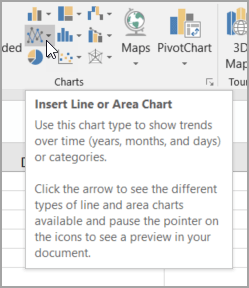
3. Click the Insert tab, and and so click Insert Line or Area Chart.

   

4. Click Line with Markers.

5. Click the nautical chart area of the chart to display the Design and Format tabs.

6. Click the Pattern tab, and then click the chart way you lot want to use.

   

7. Click the chart championship and blazon the text you want.

8. To change the font size of the chart title, correct-click the championship, click Font, and then enter the size that you want in the Size box. Click OK.

9. Click the chart area of the chart.

10. On the chart, click the legend, or add together information technology from a list of chart elements (on the Blueprint tab, click Add Chart Element > Legend, so select a location for the legend).

    

11. To plot one of the data series along a secondary vertical axis, click the data series, or select information technology from a list of chart elements (on the Format tab, in the Electric current Selection group, click Chart Elements).

    

12. On the Format tab, in the Current Selection group, click Format Pick. The Format Information Series task pane appears.

13. Under Serial Options, select Secondary Centrality, and and so click Close.

14. On the Blueprint tab, in the Chart Layouts grouping, click Add together Chart Element, and then do the following:

    1. To add a chief vertical axis title, click Axis Championship >Primary Vertical. then on the Format Axis Championship pane, click Size & Properties to configure the type of vertical centrality title that yous want.

    2. To add a secondary vertical axis championship, click Axis Championship > Secondary Vertical, and and then on the Format Centrality Title pane, click Size & Properties to configure the type of vertical axis title that you want.

    3. Click each title, type the text that you desire, and then press Enter

15. Click the plot area of the chart, or select information technology from a list of chart elements (Format tab, Current Selection group, Chart Elements box).

16. On the Format tab, in the Shape Styles group, click the More than push button , and so click the effect that you want to use.

    

17. Click the nautical chart area of the chart.

18. On the Format tab, in the Shape Styles group, click the More push , then click the issue that you lot want to utilise.

19. If you want to utilize theme colors that are different from the default theme that is applied to your workbook, exercise the post-obit:

    1. On the Page Layout tab, in the Themes grouping, click Themes.

       

    2. Under Function, click the theme that y'all want to apply.

Create a scatter or line nautical chart in Office 2010

So, how did nosotros create this scatter nautical chart? The post-obit procedure volition aid yous create a besprinkle chart with similar results. For this chart, we used the example worksheet data. Yous tin copy this data to your worksheet, or you can apply your own information.

1. Re-create the example worksheet data into a bare worksheet, or open the worksheet that contains the data that you want to plot into a besprinkle chart.

   1 2 3 4 five 6 7 eight ix x 11

   A B Daily Rainfall Particulate four.1 122 4.3 117 v.7 112 5.4 114 5.ix 110 5.0 114 iii.vi 128 1.nine 137 7.3 104

2. Select the data that you want to plot in the scatter chart.

3. On the Insert tab, in the Charts group, click Scatter.

   

4. Click Besprinkle with only Markers.

   Tip:You lot can remainder the mouse on whatsoever nautical chart blazon to see its name.

5. Click the chart area of the chart.

   This displays the Chart Tools, calculation the Pattern, Layout, and Format tabs.

6. On the Design tab, in the Chart Styles grouping, click the chart way that you want to use.

   

   For our besprinkle chart, we used Style 26.

7. On the Layout tab, click Chart Title and and then select a location for the title from the drop-down list.

   Nosotros chose Above Chart.

8. Click the chart title, and and then blazon the text that you lot want.

   For our besprinkle nautical chart, we typed Particulate Levels in Rainfall.

9. To reduce the size of the chart title, right-click the title, and then enter the size that you want in the Font Size box on the shortcut carte du jour.

   For our scatter chart, we used 14.

10. Click the chart area of the chart.

11. On the Layout tab, in the Labels grouping, click Axis Titles, and then do the post-obit:

    1. To add a horizontal axis championship, click Primary Horizontal Axis Title, and then click Title Below Axis.

    2. To add a vertical axis title, click Chief Vertical Axis Championship, and then click the blazon of vertical centrality title that you want.

       For our scatter chart, we used Rotated Title.

       

    3. Click each championship, type the text that you want, then printing Enter.

       For our scatter chart, we typed Daily Rainfall in the horizontal axis title, and Particulate level in the vertical centrality title.

12. Click the plot area of the chart, or select Plot Area from a list of chart elements (Layout tab, Current Selection grouping, Chart Elements box).

13. On the Format tab, in the Shape Styles group, click the More button , and and so click the consequence that you want to use.

    For our besprinkle chart, we used the Subtle Outcome - Accent three.

    

14. Click the chart area of the nautical chart.

15. On the Format tab, in the Shape Styles group, click the More button , and then click the effect that you lot want to use.

    For our scatter nautical chart, we used the Subtle Effect - Accent 1.

16. If you want to utilize theme colors that are dissimilar from the default theme that is applied to your workbook, practise the following:

    1. On the Page Layout tab, in the Themes group, click Themes.

       

    2. Under Born, click the theme that you want to utilize.

       For our line nautical chart, we used the Role theme.

So, how did we create this line chart? The following procedure will assist you create a line chart with similar results. For this chart, we used the example worksheet data. You can copy this data to your worksheet, or you can utilise your own data.

1. Copy the instance worksheet information into a blank worksheet, or open the worksheet that contains the data that you want to plot into a line nautical chart.

   1 2 3 four v half dozen 7 8 9 10 11

   A B C Date Daily Rainfall Particulate ane/1/07 4.1 122 1/2/07 4.3 117 i/3/07 five.vii 112 1/4/07 five.iv 114 1/v/07 5.9 110 1/six/07 five.0 114 1/7/07 3.6 128 one/eight/07 i.9 137 ane/ix/07 7.3 104

2. Select the data that you want to plot in the line chart.

3. On the Insert tab, in the Charts group, click Line.

   

4. Click Line with Markers.

5. Click the nautical chart area of the chart.

   This displays the Chart Tools, adding the Design, Layout, and Format tabs.

6. On the Blueprint tab, in the Chart Styles group, click the nautical chart way that you want to use.

   

   For our line chart, we used Way two.

7. On the Layout tab, in the Labels group, click Nautical chart Title, and then click To a higher place Nautical chart.

   

8. Click the nautical chart title, and then type the text that you desire.

   For our line chart, we typed Particulate Levels in Rainfall.

9. To reduce the size of the chart title, right-click the championship, and then enter the size that you lot want in the Size box on the shortcut menu.

   For our line chart, nosotros used 14.

10. On the chart, click the legend, or select it from a list of nautical chart elements (Layout tab, Current Selection group, Chart Elements box).

11. On the Layout tab, in the Labels group, click Legend, and then click the position that you want.

    For our line chart, we used Bear witness Legend at Top.

12. To plot one of the data serial forth a secondary vertical axis, click the data series for Rainfall, or select it from a list of chart elements (Layout tab, Electric current Selection group, Nautical chart Elements box).

13. On the Layout tab, in the Current Pick grouping, click Format Selection.

    

14. Nether Series Options, select Secondary Axis, and so click Close.

15. On the Layout tab, in the Labels group, click Axis Titles, and then do the following:

    1. To add together a primary vertical centrality championship, click Primary Vertical Centrality Title, and and then click the blazon of vertical centrality title that you desire.

       For our line chart, we used Rotated Title.

    2. To add a secondary vertical centrality title, click Secondary Vertical Axis Title, and so click the type of vertical centrality title that you desire.

       For our line nautical chart, we used Rotated Title.

    3. Click each title, type the text that y'all desire, and then press ENTER.

       For our line chart, we typed Particulate level in the primary vertical axis championship, and Daily Rainfall in the secondary vertical axis title.

16. Click the plot area of the chart, or select it from a listing of nautical chart elements (Layout tab, Current Pick group, Chart Elements box).

17. On the Format tab, in the Shape Styles grouping, click the More than button , and and then click the effect that you want to use.

    For our line chart, we used the Subtle Effect - Dark 1.

    

18. Click the chart area of the chart.

19. On the Format tab, in the Shape Styles group, click the More than button , then click the effect that you desire to use.

    For our line chart, nosotros used the Subtle Effect - Accent 3.

20. If yous want to use theme colors that are different from the default theme that is applied to your workbook, exercise the following:

    1. On the Page Layout tab, in the Themes group, click Themes.

       

    2. Under Congenital-in, click the theme that you want to use.

       For our line chart, nosotros used the Part theme.

How To Add Lines To A Scatter Plot On Excel,

Source: https://support.microsoft.com/en-us/topic/present-your-data-in-a-scatter-chart-or-a-line-chart-4570a80f-599a-4d6b-a155-104a9018b86e

Posted by: isaacslact1943.blogspot.com

Share this post